41 excel pie chart labels inside
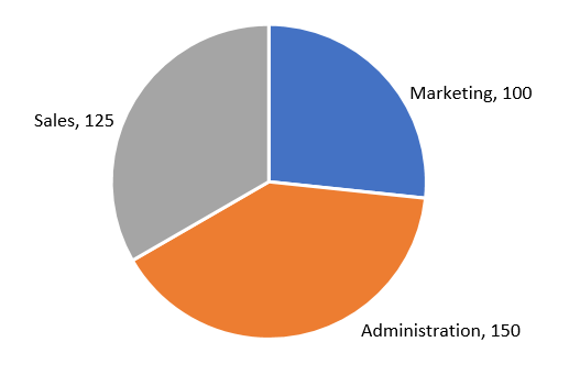
How to Make Pie of Pie Chart in Excel (with Easy Steps) Step-01: Inserting Pie of Pie Chart in Excel Firstly, you must select the data range. Here, I have selected the range B4:C12. Secondly, you have to go to the Insert tab. Now, from the Insert tab >> you need to select Insert Pie or Doughnut Chart. Then, from 2-D Pie >> you must choose Pie of Pie. How to Make a PIE Chart in Excel (Easy Step-by-Step Guide) Creating a Pie Chart in Excel. To create a Pie chart in Excel, you need to have your data structured as shown below. The description of the pie slices should be in the left column and the data for each slice should be in the right column. Once you have the data in place, below are the steps to create a Pie chart in Excel: Select the entire dataset
Creating Pie Chart and Adding/Formatting Data Labels (Excel) Creating Pie Chart and Adding/Formatting Data Labels (Excel)

Excel pie chart labels inside
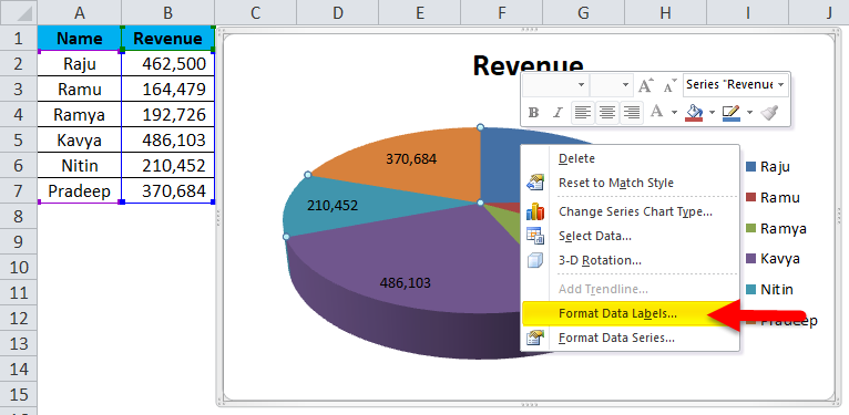
Put labels inside pie chart | MrExcel Message Board Dec 2, 2003. #2. Select and Format the data labels using the Label Position setting on the Alignment tab. N. How-to Make a WSJ Excel Pie Chart with Labels Both Inside and Outside ... How-to Make an Excel Pie Chart with Labels where the labels are both Inside and Outside of the pie slices. This... Pie Chart in Excel - Inserting, Formatting, Filters, Data Labels To insert a Pie Chart, follow these steps:- Select the range of cells A1:B7 Go to Insert tab. In the charts group, Select the pie chart button Click on pie chart in 2D chart section. Adding Data Labels The default pie chart inserted in the above section is:-
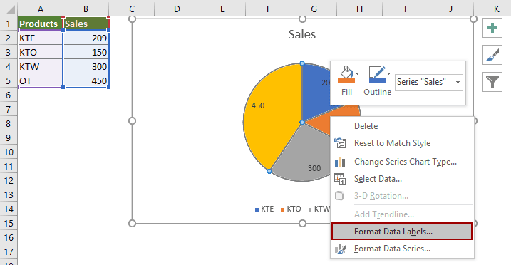
Excel pie chart labels inside. How to create pie of pie or bar of pie chart in Excel? - ExtendOffice Then you can add the data labels for the data points of the chart, please select the pie chart and right click, then choose Add Data Labels from the context menu and the data labels are appeared in the chart. See screenshots: And now the labels are added for each data point. See screenshot: 5. Go on selecting the pie chart and right clicking, then choose Format Data Series from the context menu, see screenshot: 6. text within a data label in pie chart in excel 2010 doesn't align Right-click a data label. Choose Format Data Labels. Click "Label Options" at top. "Label position" options in bottom half of dialog box. -OR-. Click "Alignment" at bottom. "Alignment options" at top of dialog box. '---. Jim Cone. Add or remove data labels in a chart - support.microsoft.com Click the data series or chart. To label one data point, after clicking the series, click that data point. In the upper right corner, next to the chart, click Add Chart Element > Data Labels. To change the location, click the arrow, and choose an option. If you want to show your data label inside a text bubble shape, click Data Callout. Move data labels - support.microsoft.com Click any data label once to select all of them, or double-click a specific data label you want to move. Right-click the selection > Chart Elements > Data Labels arrow, and select the placement option you want. Different options are available for different chart types. For example, you can place data labels outside of the data points in a pie chart but not in a column chart.
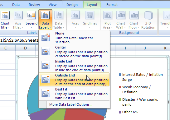
How to Make a 2010 Excel Pie Chart with Labels Both Inside and Outside ... I am following the instructions in this article: . I am following all steps until step #9 - 9) Move Second Series to the Secondary Axis - when I bring up the Format Series Dialog box - Series Options - I do not see the option to plot the series on the primary or secondary axis. Pie Chart in Excel | How to Create Pie Chart - EDUCBA Step 1: Select the data to go to Insert, click on PIE, and select 3-D pie chart. Step 2: Now, it instantly creates the 3-D pie chart for you. Step 3: Right-click on the pie and select Add Data Labels. This will add all the values we are showing on the slices of the pie. How to insert data labels to a Pie chart in Excel 2013 - YouTube This video will show you the simple steps to insert Data Labels in a pie chart in Microsoft® Excel 2013. Office: Display Data Labels in a Pie Chart - Tech-Recipes: A Cookbook ... This will typically be done in Excel or PowerPoint, but any of the Office programs that supports charts will allow labels through this method. 1. Launch PowerPoint, and open the document that you want to edit. 2. If you have not inserted a chart yet, go to the Insert tab on the ribbon, and click the Chart option. 3. In the Chart window, choose the Pie chart option from the list on the left. Next, choose the type of pie chart you want on the right side. 4.
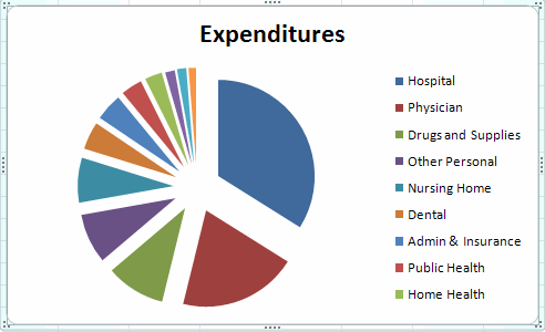
Pie of Pie Chart in Excel - Inserting, Customizing - Excel Unlocked To insert a Pie of Pie chart:- Select the data range A1:B7. Enter in the Insert Tab. Select the Pie button, in the charts group. Select Pie of Pie chart in the 2D chart section. Adding Data Labels to Pie of Pie Chart The chart inserted in the above section is:- Pie in a Pie Chart - Excel Master Constructing the PIP Chart Drawing a pip chart is the same as drawing almost any other chart: select the data, click Insert, click Charts and then choose the chart style you want. In this case, the chart we want is this one … That is, choose the middle of the three pies shown under the heading 2-D Pie. That's it! That's all you do. Excel Pie Chart - How to Create & Customize? (Top 5 Types) We will customize the Pie Chart in Excel by Adding Data Labels. Scenario 1: The procedure to add data labels are as follows: Click on the Pie Chart > click the '+' icon > check/tick the "Data Labels" checkbox in the "Chart Element" box > select the "Data Labels" right arrow > select the "Outside End" option. We get the following output. How to Make a Pie Chart in Excel & Add Rich Data Labels to The Chart! Creating and formatting the Pie Chart. 1) Select the data. 2) Go to Insert> Charts> click on the drop-down arrow next to Pie Chart and under 2-D Pie, select the Pie Chart, shown below. 3) Chang the chart title to Breakdown of Errors Made During the Match, by clicking on it and typing the new title.
Add or remove data labels in a chart
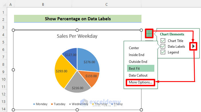
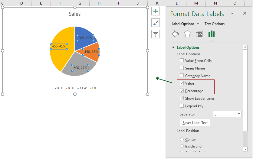
Change the format of data labels in a chart To get there, after adding your data labels, select the data label to format, and then click Chart Elements > Data Labels > More Options. To go to the appropriate area, click one of the four icons (Fill & Line, Effects, Size & Properties (Layout & Properties in Outlook or Word), or Label Options) shown here.
How to fix wrapped data labels in a pie chart | Sage Intelligence
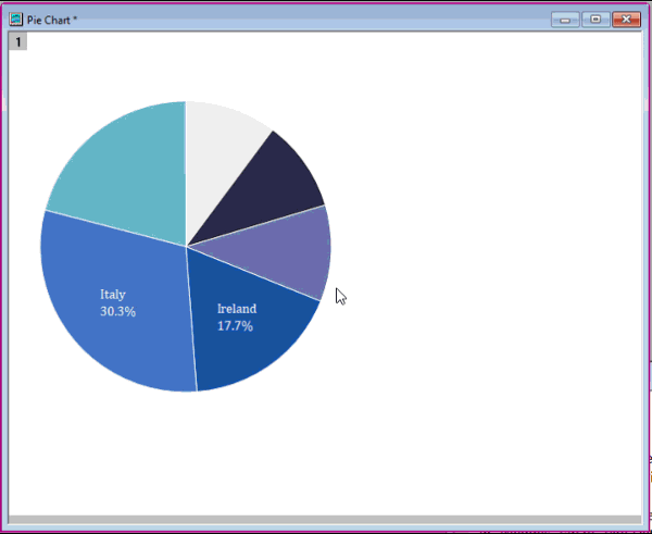
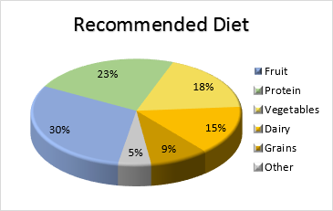
How to Create and Format a Pie Chart in Excel - Lifewire Drag a data label to reposition it inside a slice. To explode a slice of a pie chart: Select the plot area of the pie chart. Select a slice of the pie chart to surround the slice with small blue highlight dots. Drag the slice away from the pie chart to explode it. To reposition a data label, select the data label to select all data labels.

Chart Data Labels in PowerPoint 2013 for Windows
Pie Chart in Excel - Inserting, Formatting, Filters, Data Labels To insert a Pie Chart, follow these steps:- Select the range of cells A1:B7 Go to Insert tab. In the charts group, Select the pie chart button Click on pie chart in 2D chart section. Adding Data Labels The default pie chart inserted in the above section is:-

How to show percentages on three different charts in Excel ...
How-to Make a WSJ Excel Pie Chart with Labels Both Inside and Outside ... How-to Make an Excel Pie Chart with Labels where the labels are both Inside and Outside of the pie slices. This...
How to Edit Pie Chart in Excel (All Possible Modifications ...
Put labels inside pie chart | MrExcel Message Board Dec 2, 2003. #2. Select and Format the data labels using the Label Position setting on the Alignment tab. N.

How to make a pie chart in Excel
Label inside donut chart · Issue #78 · chartjs/Chart.js · GitHub

Excel: How to not display labels in pie chart that are 0 ...

How to data label on pie chart? - Simple Excel VBA
How to show percentage in pie chart in Excel?

Display Data and Percentage in Pie Chart | SAP Blogs
Help Online - Quick Help - FAQ-1017 How to recover the ...

How to Change Excel Chart Data Labels to Custom Values?

How to insert data labels to a Pie chart in Excel 2013

Change the format of data labels in a chart
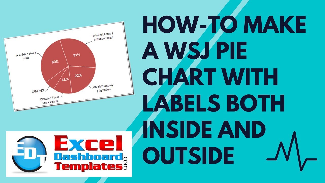
How-to Make a WSJ Excel Pie Chart with Labels Both Inside and Outside

How to show data labels in PowerPoint and place them ...
information graphics - How to display data labels in ...
Is there a way to prevent pie chart data labels from ...
How to Make Pie Chart with Labels both Inside and Outside ...
/Capture-5c8489fbc9e77c0001422f49.JPG)
How to Create and Format a Pie Chart in Excel

Create Outstanding Pie Charts in Excel | Pryor Learning

How to Make an Excel Pie Chart

Change the format of data labels in a chart

How to Make Pie Charts in ggplot2 (With Examples)
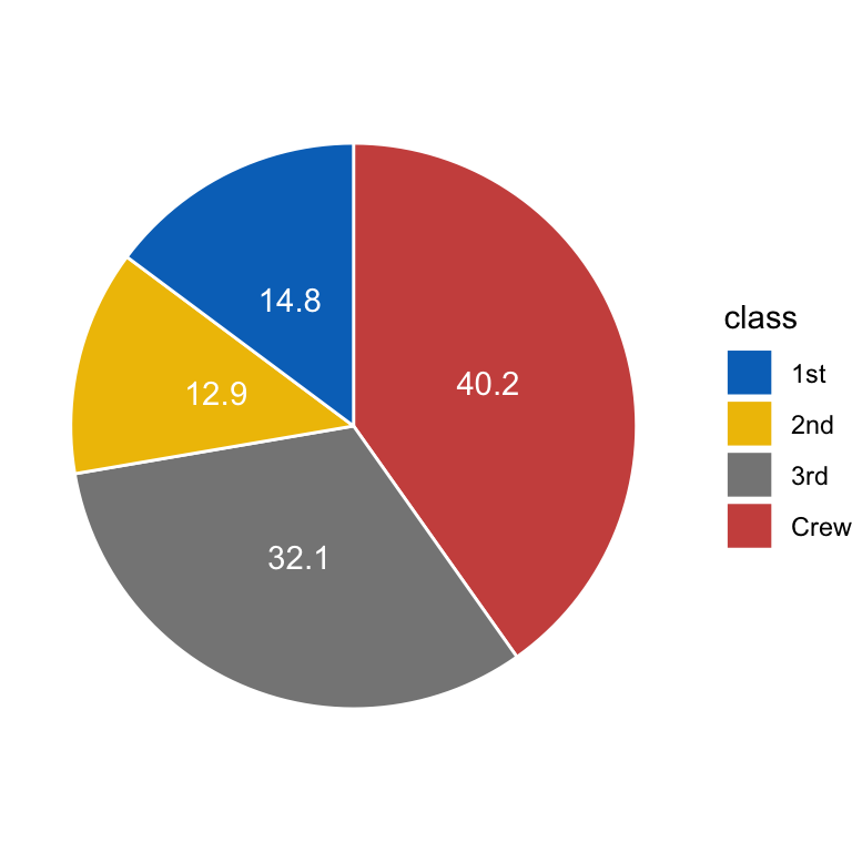
How to Create a Pie Chart in R using GGPLot2 - Datanovia

Remake: Pie-in-a-Donut Chart - PolicyViz

How to make a pie chart in Excel

Optimally positioning pie chart data labels in Excel with VBA ...
How-to Make a WSJ Excel Pie Chart with Labels Both Inside and ...
EXCEL Charts: Column, Bar, Pie and Line

Power BI Pie Chart - Complete Tutorial - SPGuides

Pie charts - Google Docs Editors Help

How to Make Pie Chart with Labels both Inside and Outside ...
How to show percentage in pie chart in Excel?

How to show percentage in pie chart in Excel?

How to make a pie chart in Excel

Display Total Inside Power BI Donut Chart | John Dalesandro
How to make a pie chart in Excel
Pie Chart in Excel | How to Create Pie Chart | Step-by-Step ...

How to Create a Pie Chart in Excel | Smartsheet
Post a Comment for "41 excel pie chart labels inside"