40 how to add data labels to a pie chart in excel on mac

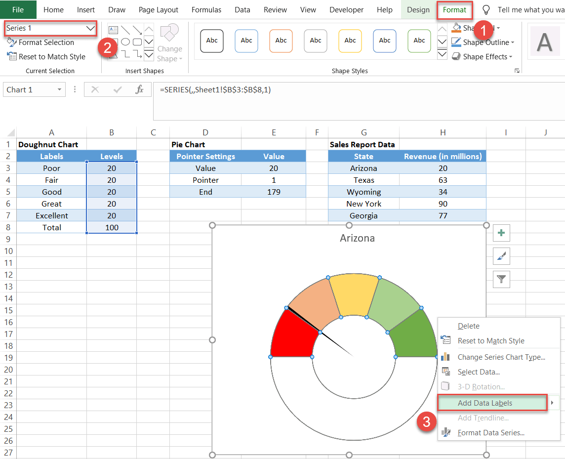
How to Create and Format a Pie Chart in Excel - Lifewire To add data labels to a pie chart: Select the plot area of the pie chart. Right-click the chart. Select Add Data Labels . Select Add Data Labels. In this example, the sales for each cookie is added to the slices of the pie chart. Change Colors How to Insert Axis Labels In An Excel Chart | Excelchat We will again click on the chart to turn on the Chart Design tab. We will go to Chart Design and select Add Chart Element. Figure 6 - Insert axis labels in Excel. In the drop-down menu, we will click on Axis Titles, and subsequently, select Primary vertical. Figure 7 - Edit vertical axis labels in Excel. Now, we can enter the name we want ...

Create a chart in Excel for Mac - support.microsoft.com Click a specific chart type and select the style you want. With the chart selected, click the Chart Design tab to do any of the following: Click Add Chart Element to modify details like the title, labels, and the legend. Click Quick Layout to choose from predefined sets of chart elements.

How to add data labels to a pie chart in excel on mac

Office: Display Data Labels in a Pie Chart - Tech-Recipes: A Cookbook ... 2. If you have not inserted a chart yet, go to the Insert tab on the ribbon, and click the Chart option. 3. In the Chart window, choose the Pie chart option from the list on the left. Next, choose the type of pie chart you want on the right side. 4. Once the chart is inserted into the document, you will notice that there are no data labels. How to Create Pie Charts in Excel (In Easy Steps) - Excel Easy Select the range A1:D1, hold down CTRL and select the range A3:D3. 6. Create the pie chart (repeat steps 2-3). 7. Click the legend at the bottom and press Delete. 8. Select the pie chart. 9. Click the + button on the right side of the chart and click the check box next to Data Labels. › 07 › 09Rotate charts in Excel - spin bar, column, pie and line ... Jul 09, 2014 · After being rotated my pie chart in Excel looks neat and well-arranged. Thus, you can see that it's quite easy to rotate an Excel chart to any angle till it looks the way you need. It's helpful for fine-tuning the layout of the labels or making the most important slices stand out. Rotate 3-D charts in Excel: spin pie, column, line and bar charts

How to add data labels to a pie chart in excel on mac. Change the look of chart text and labels in Numbers on Mac If you can't edit a chart, you may need to unlock it. Change the font, style, and size of chart text Edit the chart title Add and modify chart value labels Add and modify pie chart wedge labels or donut chart segment labels Modify axis labels Edit pivot chart data labels Note: Axis options may be different for scatter and bubble charts. Add a DATA LABEL to ONE POINT on a chart in Excel - Excel Quick Help All the data points will be highlighted. Click again on the single point that you want to add a data label to. Right-click and select ' Add data label '. This is the key step! Right-click again on the data point itself (not the label) and select ' Format data label '. You can now configure the label as required — select the content of ... Pie Chart in Excel | How to Create Pie Chart - EDUCBA Step 1: Do not select the data; rather, place a cursor outside the data and insert one PIE CHART. Go to the Insert tab and click on a PIE. Step 2: once you click on a 2-D Pie chart, it will insert the blank chart as shown in the below image. Step 3: Right-click on the chart and choose Select Data. Add column, bar, line, area, pie, donut, and radar charts in Numbers on Mac Create a column, bar, line, area, pie, donut, or radar chart. Click in the toolbar, then click 2D, 3D, or Interactive. Click the left and right arrows to see more styles. Note: The stacked bar, column, and area charts show two or more data series stacked together. Click a chart or drag it to the sheet. If you add a 3D chart, you see at its center.

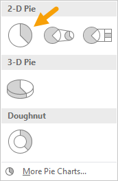
Excel custom pie chart labels - Microsoft Community Excel custom pie chart labels. I want to use a pivot table to make a pie chart out of this. I want each of the pieces of the pie to contain the number of entries and between parentheses the percentage. So in the "Yes" piece, there should be '3 (33%)'. Actually, if I hover the pie chart in Excel, I get exactly the notation O want! support.microsoft.com › en-us › officeAdd or remove data labels in a chart - support.microsoft.com For example, in the pie chart below, without the data labels it would be difficult to tell that coffee was 38% of total sales. Depending on what you want to highlight on a chart, you can add labels to one series, all the series (the whole chart), or one data point. Add data labels. You can add data labels to show the data point values from the ... How to show percentage in pie chart in Excel? - ExtendOffice Select the data you will create a pie chart based on, click Insert > I nsert Pie or Doughnut Chart > Pie. See screenshot: 2. Then a pie chart is created. Right click the pie chart and select Add Data Labels from the context menu. 3. Now the corresponding values are displayed in the pie slices. How to Make a Pie Chart in Excel: 10 Steps (with Pictures) - wikiHow If you would rather make a chart from data you already have, double-click the Excel document that contains the data to open it and proceed to the next section. 2 Click Blank workbook (PC) or Excel Workbook (Mac). It's in the top-left side of the "Template" window. 3 Add a name to the chart.

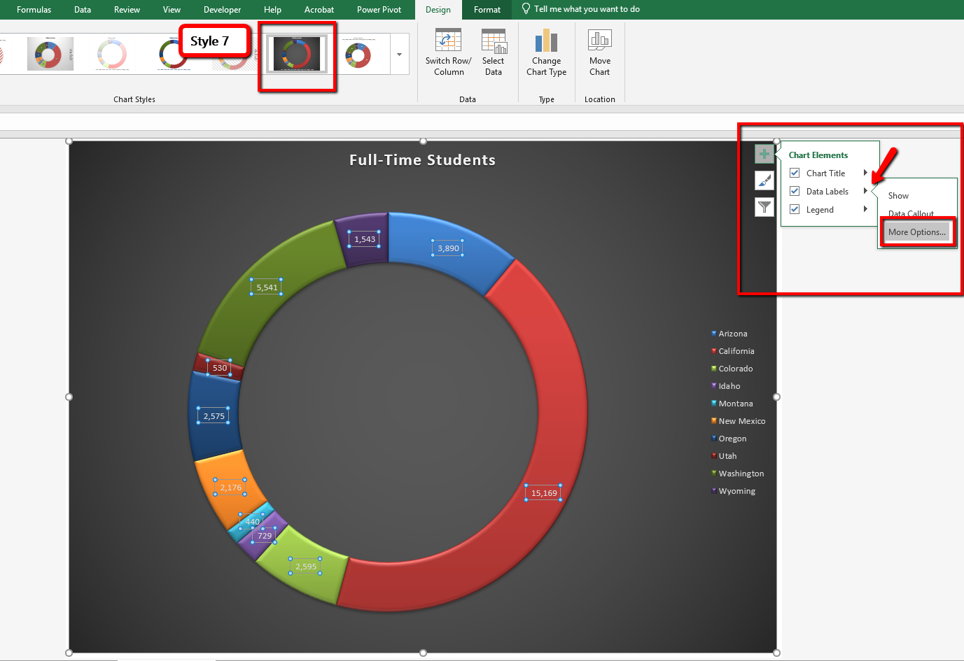
Add a Data Callout Label to Charts in Excel 2013 - Software Tips and Tricks In the upper right corner, next to your chart, click the Chart Elements button (plus sign), and then click Data Labels. A right pointing arrow will appear, click on this arrow to view the submenu. Select Data Callout. Once the Data Callout Labels have been added, you can re-position them by clicking on their borders and dragging to a new position. How to add percentage to pie chart in excel - kasapwestcoast To add data labels, select the chart and then click on the + button in the top right corner of the pie chart and check the Data Labels button. Initially, the pie chart will not have any data labels in it. Select -> Insert -> Doughnut or Pie Chart -> 2-D Pie. Open Microsoft Excel and select the data that you want to create a pie. support.apple.com › guide › numbersImport an Excel or text file into Numbers on Mac - Apple Support Add or delete a chart. Select data to make a chart; Add column, bar, line, area, pie, donut, and radar charts; Add scatter and bubble charts; Interactive charts; Delete a chart; Change a chart’s type; Modify chart data; Move and resize charts; Change the look of a chart. Change the look of data series; Add a legend, gridlines, and other ... How to display leader lines in pie chart in Excel? - ExtendOffice To display leader lines in pie chart, you just need to check an option then drag the labels out. 1. Click at the chart, and right click to select Format Data Labels from context menu. 2. In the popping Format Data Labels dialog/pane, check Show Leader Lines in the Label Options section. See screenshot: 3.

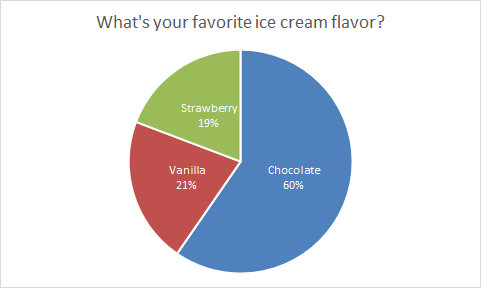
Pie Chart: Survey results favorite ice cream flavor | Exceljet

How to Make a PIE Chart in Excel (Easy Step-by-Step Guide) - Trump Excel Here are the steps to format the data label from the Design tab: Select the chart. This will make the Design tab available in the ribbon. In the Design tab, click on the Add Chart Element (it's in the Chart Layouts group). Hover the cursor on the Data Labels option.

Excel Gauge Chart Template - Free Download - How to Create

How to Make a Pie Chart in Excel — Everything You Need to Know 3. Select the first cell and drag cursor till the last cell to select whole data. 4. Click Insert > Pie. 5. A pie chart will automatically appear. 6. To enter the title of chart, click on highlighted area. 7. Enter your chart's title. Editing Your Pie-Chart Labeling. 1. The labels/values exist as automatically selected. Right-click anywhere ...

Pie Chart: Survey results favorite ice cream flavor | Exceljet

How to Add Data Labels to an Excel 2010 Chart - dummies Use the following steps to add data labels to series in a chart: Click anywhere on the chart that you want to modify. On the Chart Tools Layout tab, click the Data Labels button in the Labels group. A menu of data label placement options appears: None: The default choice; it means you don't want to display data labels.

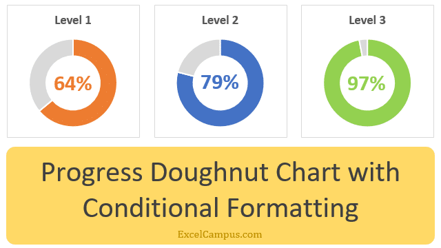
Charts & Dashboards Archives - Page 2 of 5 - Excel Campus

› pie-chartPie Charts: Types, Advantages, Examples, and More - Edrawsoft In this article, you will know how to create a pie chart in Excel and on EdrawMax as well. 1. Pie Chart in Excel . Making a pie chart in Excel can be very easy if you correctly follow the step-by-step tutorial below. For instance, you are making a pie chart in Excel representing the percentage of people who own certain types of pets:

4.1 Choosing a Chart Type – Beginning Excel 2019

How to Create a Pie Chart in Excel - Smartsheet If want the category names to appear on or near the chart, right-click on the chart and click Add Data Labels …. By default, the numerical values are added. To add other labels, such as the categorical values or the percentage of the total that each category represents, right-click on the chart, then click Format Data Labels ….

33 How To Label A Pie Chart In Excel - Labels 2021

› data-definition-excel-3123415Excel Spreadsheet Data Types - Lifewire Feb 07, 2020 · Text data, also called labels, is used for worksheet headings and names that identify columns of data. Text data can contain letters, numbers, and special characters such as ! or &. By default, text data is left-aligned in a cell. Number data, also called values, is used in calculations. By default, numbers are right-aligned in a cell.

33 How To Label A Pie Chart In Excel - Labels 2021

Formatting data labels and printing pie charts on Excel for Mac 2019 ... Work around: Select the area of the chart - by selecting the cells behind where the chart is sitting > Print area> Select print area>File > print>then set print perameters (paper size, fit to page etc.) > Print. This worked. 2. When formatting data labels on an extended bar of pie chart: Excel does not allow me to:

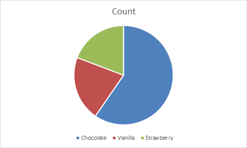
Pie Chart: Survey results favorite ice cream flavor | Exceljet

How to make a pie chart in Excel - ablebits.com To rotate a pie chart in Excel, do the following: Right-click any slice of your pie graph and click Format Data Series. On the Format Data Point pane, under Series Options, drag the Angle of first slice slider away from zero to rotate the pie clockwise. Or, type the number you want directly in the box.

Share :