39 excel chart rotate axis labels

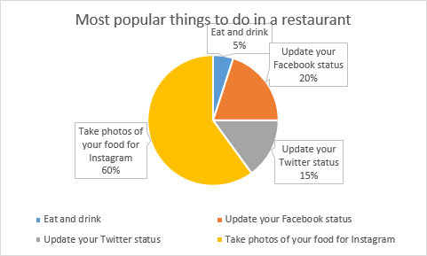
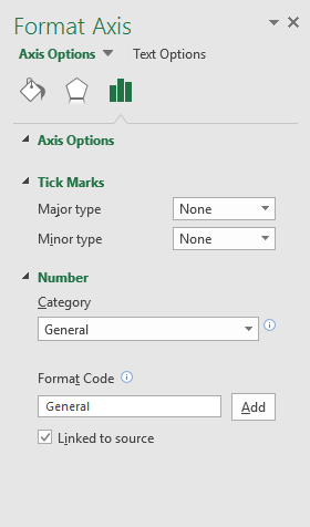
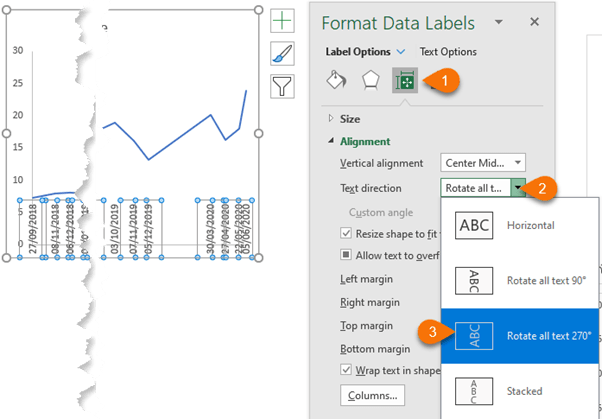
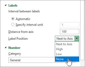
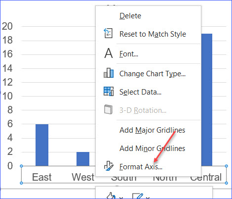
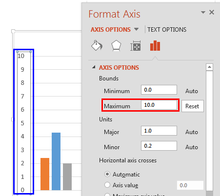
› how-to-show-percentage-inHow to Show Percentage in Pie Chart in Excel? - GeeksforGeeks Jun 29, 2021 · To add data labels, select the chart and then click on the “+” button in the top right corner of the pie chart and check the Data Labels button. Pie Chart It can be observed that the pie chart contains the value in the labels but our aim is to show the data labels in terms of percentage. › documents › excelHow to rotate axis labels in chart in Excel? - ExtendOffice 1. Right click at the axis you want to rotate its labels, select Format Axis from the context menu. See screenshot: 2. In the Format Axis dialog, click Alignment tab and go to the Text Layout section to select the direction you need from the list box of Text direction. See screenshot: 3. Close the dialog, then you can see the axis labels are ...

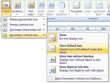
› charts › secondary-axisHow to Add Secondary Axis (X & Y) in Excel & Google Sheets 4. Under Series where it says, Apply to all Series, change this to the series you want on the secondary axis. In this case, we’ll select “Net Income” 5. Scroll down under Axis and Select Right Axis . Final Graph with Secondary Axis. Now the final graph shows the Revenue on the Primary (left) axis and the Net Income on the Secondary (right ...

Excel chart rotate axis labels

› charts › thermometer-templateExcel Thermometer Chart – Free Download & How to Create Right-click on the data label and choose “Format Data Labels.” Then, in the Label Options tab, under Label Position, choose “Inside End.” Step #8: Move Series 1 “Target Revenue” to the secondary axis. To mold the chart into a thermometer shape, you need to get Series 1 “Target Revenue” (E2) in the right position. › charts › axis-textChart Axis – Use Text Instead of Numbers - Automate Excel 8. Select XY Chart Series. 9. Click Edit . 10. Select X Value with the 0 Values and click OK. Change Labels. While clicking the new series, select the + Sign in the top right of the graph; Select Data Labels; Click on Arrow and click Left . 4. Double click on each Y Axis line type = in the formula bar and select the cell to reference . 5. support.microsoft.com › en-us › officeRotate a pie chart - support.microsoft.com If you want to rotate another type of chart, such as a bar or column chart, you simply change the chart type to the style that you want. For example, to rotate a column chart, you would change it to a bar chart. Select the chart, click the Chart Tools Design tab, and then click Change Chart Type. See Also. Add a pie chart. Available chart types ...

Excel chart rotate axis labels. › pie-chart-examplesPie Chart Examples | Types of Pie Charts in Excel ... - EDUCBA This is a guide to Pie Chart Examples. Here we discuss Types of Pie Chart in Excel along with practical examples and downloadable excel template. You can also go through our other suggested articles – Excel Combination Charts; Chart Wizard in Excel; Pie Chart in Excel; Pie Chart In MS Excel support.microsoft.com › en-us › officeRotate a pie chart - support.microsoft.com If you want to rotate another type of chart, such as a bar or column chart, you simply change the chart type to the style that you want. For example, to rotate a column chart, you would change it to a bar chart. Select the chart, click the Chart Tools Design tab, and then click Change Chart Type. See Also. Add a pie chart. Available chart types ... › charts › axis-textChart Axis – Use Text Instead of Numbers - Automate Excel 8. Select XY Chart Series. 9. Click Edit . 10. Select X Value with the 0 Values and click OK. Change Labels. While clicking the new series, select the + Sign in the top right of the graph; Select Data Labels; Click on Arrow and click Left . 4. Double click on each Y Axis line type = in the formula bar and select the cell to reference . 5. › charts › thermometer-templateExcel Thermometer Chart – Free Download & How to Create Right-click on the data label and choose “Format Data Labels.” Then, in the Label Options tab, under Label Position, choose “Inside End.” Step #8: Move Series 1 “Target Revenue” to the secondary axis. To mold the chart into a thermometer shape, you need to get Series 1 “Target Revenue” (E2) in the right position.

How to wrap X axis labels in a chart in Excel?

Customize C# Chart Options - Axis, Labels, Grouping ...

Changing Axis Labels in PowerPoint 2013 for Windows

Help Online - Origin Help - The (Plot Details) Axis Tab

Rotate x-axis (horizontal) data point text in graph to custom ...

Axis Labels in FlexChart | Axes | Wijmo Docs

How to Change Orientation of Multi-Level Labels in a Vertical ...

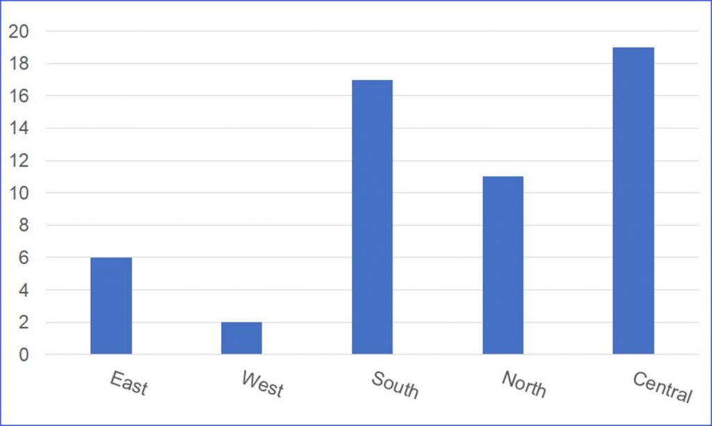
How to Rotate X Axis Labels in Chart - ExcelNotes

Excel Chart Vertical Axis Text Labels • My Online Training Hub

Rotate Axis labels in Excel - Free Excel Tutorial

Two-Level Axis Labels (Microsoft Excel)

How to align 45 degree bar chart labels to end at stick mark?

Rotate charts in Excel - spin bar, column, pie and line charts

Axis Label Alignment - Microsoft Community

Microsoft Excel: Extending the x-axis of a chart without ...

How to Customize GGPLot Axis Ticks for Great Visualization ...

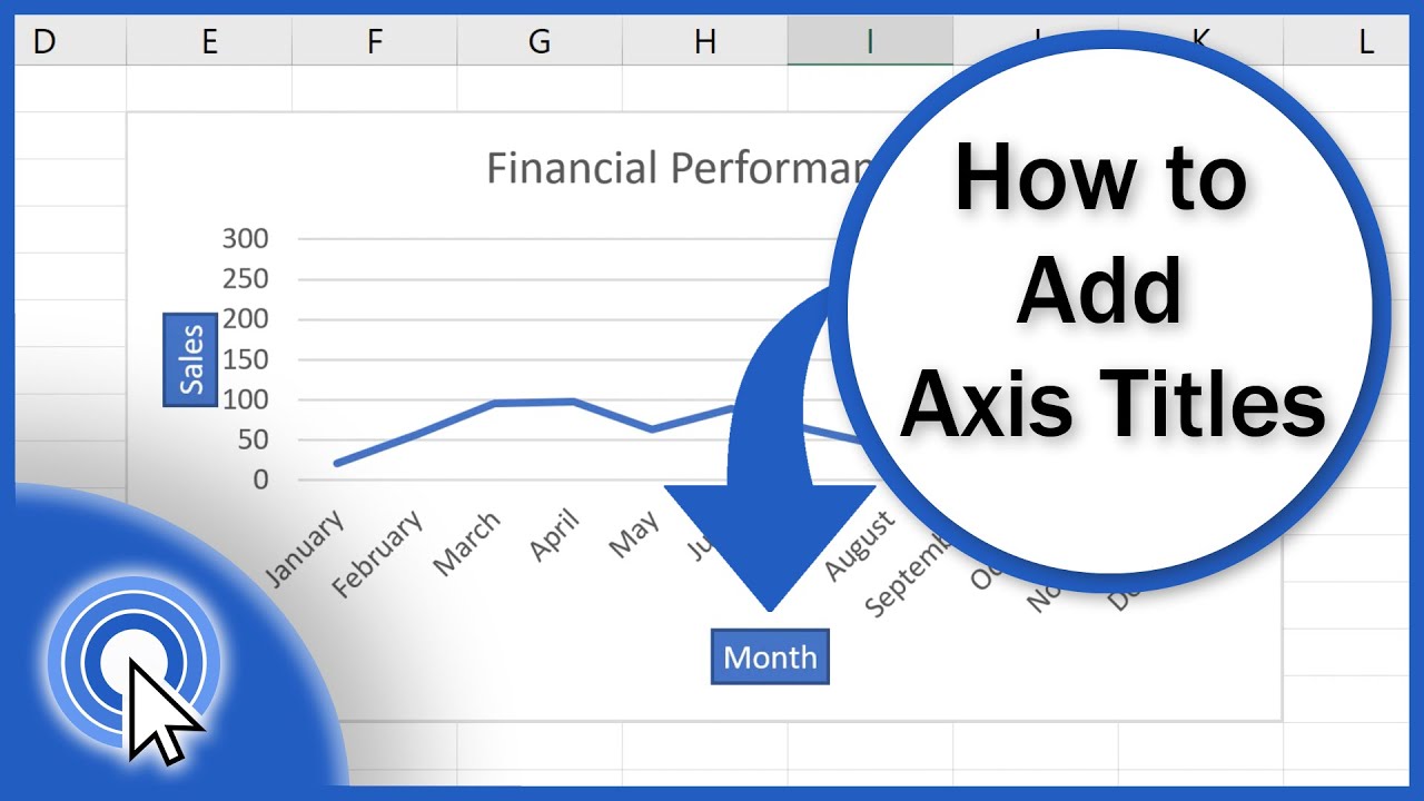
How to Add Axis Titles in Excel

Label Specific Excel Chart Axis Dates • My Online Training Hub

How To Rotate x-axis Text Labels in ggplot2 - Data Viz with ...

How to Change Orientation of Multi-Level Labels in a Vertical ...

Text Labels on a Vertical Column Chart in Excel - Peltier Tech

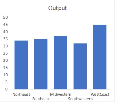
3 Ways to Make Excel Chart Horizontal Categories Fit Better ...

Change the display of chart axes

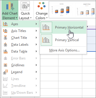
Change the display of chart axes

How to Rotate Data Labels in Excel (2 Simple Methods)

How to Rotate Axis Labels in Excel (With Example) - Statology

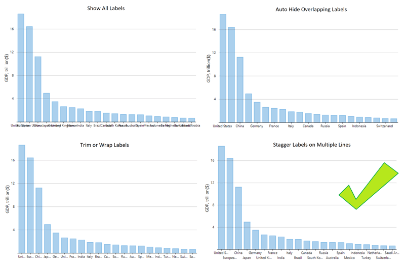
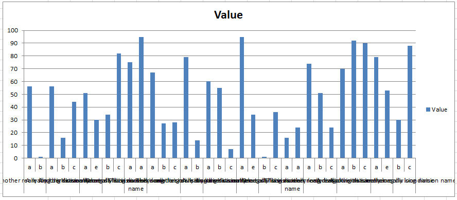
Stagger long axis labels and make one label stand out in an ...

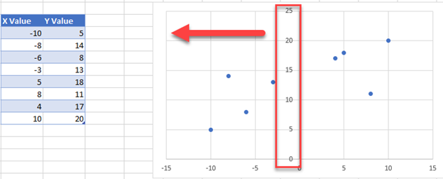
Move Vertical Axis to the Left – Excel & Google Sheets ...

Axis Titles in PowerPoint 2011 for Mac

How to Add Axis Labels in Excel Charts - Step-by-Step (2022)

How to Rotate X Axis Labels in Chart - ExcelNotes

Need to rotate category labels for 2 variables on x-axis ...

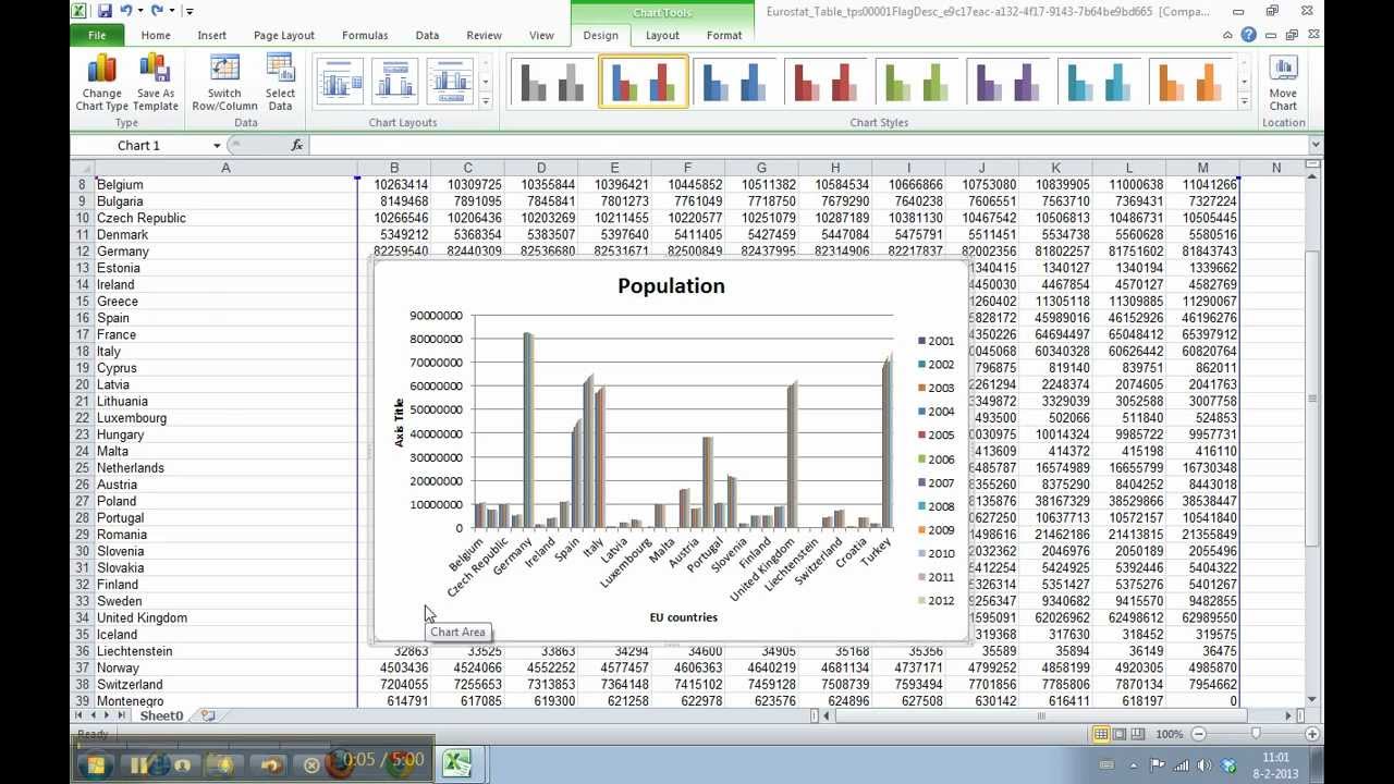
How to format the chart axis labels in Excel 2010

How To Rotate x-axis Text Labels in ggplot2 - Data Viz with ...

Display Customized Data Labels on Charts & Graphs

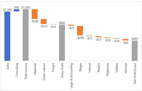
Excel Waterfall Charts • My Online Training Hub

Changing Axis Labels in PowerPoint 2013 for Windows

How to rotate axis labels in chart in Excel?

How to Rotate X Axis Labels in Chart - ExcelNotes

Share :