44 excel graph data labels

› make-a-scatter-plot-in-excelHow to Make a Scatter Plot in Excel and Present Your Data - MUO May 17, 2021 · Then select the Data Labels and click on the black arrow to open More Options. Now, click on More Options to open Label Options. Click on Select Range to define a shorter range from the data sets. Points will now show labels from column A2:A6. For a clear visualization of a label, drag the labels away as necessary. Create Dynamic Chart Data Labels with Slicers - Excel Campus 10.02.2016 · Step 5: Setup the Data Labels. The next step is to change the data labels so they display the values in the cells that contain our CHOOSE formulas. As I mentioned before, we can use the “Value from Cells” feature in Excel 2013 or 2016 to make this easier. You basically need to select a label series, then press the Value from Cells button in ...

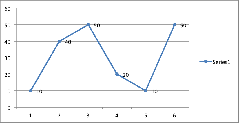
How to create Custom Data Labels in Excel Charts - Efficiency 365 Add data labels Create a simple line chart while selecting the first two columns only. Now Add Regular Data Labels. Two ways to do it. Click on the Plus sign next to the chart and choose the Data Labels option. We do NOT want the data to be shown. To customize it, click on the arrow next to Data Labels and choose More Options …

Excel graph data labels

Find, label and highlight a certain data point in Excel scatter graph 10.10.2018 · Select the Data Labels box and choose where to position the label. By default, Excel shows one numeric value for the label, y value in our case. To display both x and y values, right-click the label, click Format Data Labels…, select the X Value and Y value boxes, and set the Separator of your choosing: Label the data point by name How to Add Labels to Scatterplot Points in Excel - Statology Step 3: Add Labels to Points. Next, click anywhere on the chart until a green plus (+) sign appears in the top right corner. Then click Data Labels, then click More Options…. In the Format Data Labels window that appears on the right of the screen, uncheck the box next to Y Value and check the box next to Value From Cells. Excel tutorial: How to use data labels Generally, the easiest way to show data labels to use the chart elements menu. When you check the box, you'll see data labels appear in the chart. If you have more than one data series, you can select a series first, then turn on data labels for that series only. You can even select a single bar, and show just one data label.

Excel graph data labels. Bar Graph in Excel — All 4 Types Explained Easily - Simon Sez IT There are actually 4 types of bar graphs available in Excel. Simple bar graph which shows bars of data for one variable. Grouped bar graph which shows bars of data for multiple variables. Stacked bar graph which shows the contribution of each variable to the total. Percentage bar graph which shows the percentage of contribution to the total. How to add data labels from different column in an Excel chart? This method will guide you to manually add a data label from a cell of different column at a time in an Excel chart. 1. Right click the data series in the chart, and select Add Data Labels > Add Data Labels from the context menu to add data labels. 2. Linking a graph in PowerPoint to the Excel data so the graph can ... Set up the data required for the graph in a set of Excel cells. When you create the graph in PowerPoint, use Paste Special – Values to copy the data from Excel. You can format your graph in PowerPoint and it will be compliant with your organization’s branding standards. Because the data is in the PowerPoint file, you (or others) can update ... Excel Charts - Aesthetic Data Labels - tutorialspoint.com Data labels stay in place, even when you switch to a different type of chart. You can also connect the data labels to their data points with leader lines on all charts. Here, we will use a Bubble chart to see the formatting of data labels. Data Label Positions. To place the data labels in the chart, follow the steps given below.

How to I rotate data labels on a column chart so that they are ... To change the text direction, first of all, please double click on the data label and make sure the data are selected (with a box surrounded like following image). Then on your right panel, the Format Data Labels panel should be opened. Go to Text Options > Text Box > Text direction > Rotate Excel Graph Data Labels - Mouse Over Effects - Microsoft Community Excel; Microsoft 365 and Office; Search Community member; DB. Dyllan B. ... no, data labels in a chart will either be visible or not. A data point in a chart will show a pop up with information about the data point when the mouse is hovering over it, though. _____ cheers, teylyn ... chandoo.org › wp › change-data-labels-in-chartsHow to Change Excel Chart Data Labels to Custom Values? May 05, 2010 · Now, click on any data label. This will select “all” data labels. Now click once again. At this point excel will select only one data label. Go to Formula bar, press = and point to the cell where the data label for that chart data point is defined. Repeat the process for all other data labels, one after another. See the screencast. Add data labels and callouts to charts in Excel 365 - EasyTweaks.com Excel also gives you the option of formatting the data labels to suit your desired look if you don't like the default. To make changes to the data labels, right-click within the chart and select the "Format Labels" option. Some of the formatting options you will have include; changing the label position, changing its alignment angle, and many more.

Add a DATA LABEL to ONE POINT on a chart in Excel Steps shown in the video above: Click on the chart line to add the data point to. All the data points will be highlighted. Click again on the single point that you want to add a data label to. Right-click and select ' Add data label ' This is the key step! Right-click again on the data point itself (not the label) and select ' Format data label '. Excel charts: how to move data labels to legend @Matt_Fischer-Daly . You can't do that, but you can show a data table below the chart instead of data labels: Click anywhere on the chart. On the Design tab of the ribbon (under Chart Tools), in the Chart Layouts group, click Add Chart Element > Data Table > With Legend Keys (or No Legend Keys if you prefer) › Make-a-Line-Graph-in-Microsoft-ExcelHow to Make a Line Graph in Microsoft Excel: 12 Steps - wikiHow Jul 28, 2022 · Enter your data. A line graph requires two axes in order to function. Enter your data into two columns. For ease of use, set your X-axis data (time) in the left column and your recorded observations in the right column. For example, tracking your budget over the year would have the date in the left column and an expense in the right. How to Use Cell Values for Excel Chart Labels - How-To Geek Select the chart, choose the "Chart Elements" option, click the "Data Labels" arrow, and then "More Options." Uncheck the "Value" box and check the "Value From Cells" box. Select cells C2:C6 to use for the data label range and then click the "OK" button. The values from these cells are now used for the chart data labels.

Two-Level Axis Labels (Microsoft Excel)

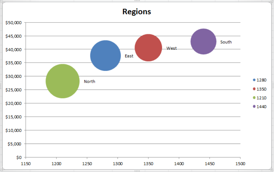
Excel: How to Create a Bubble Chart with Labels - Statology Step 3: Add Labels. To add labels to the bubble chart, click anywhere on the chart and then click the green plus "+" sign in the top right corner. Then click the arrow next to Data Labels and then click More Options in the dropdown menu: In the panel that appears on the right side of the screen, check the box next to Value From Cells within ...

How to Make Bubble Chart in Excel - Excelchat | Excelchat

How to add data labels from different column in an Excel chart? Reuse Anything: Add the most used or complex formulas, charts and anything else to your favorites, and quickly reuse them in the future. More than 20 text features: Extract Number from Text String; Extract or Remove Part of Texts; Convert Numbers and Currencies to English Words. Merge Tools: Multiple Workbooks and Sheets into One; Merge Multiple Cells/Rows/Columns …

How to Make a Bar Chart in Excel | Smartsheet

Edit titles or data labels in a chart - support.microsoft.com The first click selects the data labels for the whole data series, and the second click selects the individual data label. Right-click the data label, and then click Format Data Label or Format Data Labels. Click Label Options if it's not selected, and then select the Reset Label Text check box. Top of Page

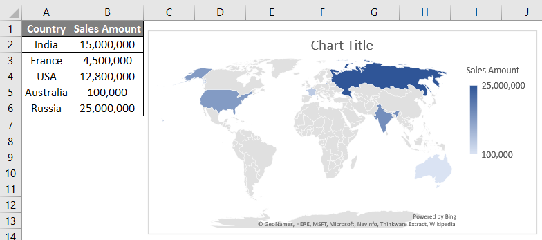
Map Chart in Excel | Steps to Create Map Chart in Excel with Examples

Custom Chart Data Labels In Excel With Formulas - How To Excel At Excel Follow the steps below to create the custom data labels. Select the chart label you want to change. In the formula-bar hit = (equals), select the cell reference containing your chart label's data. In this case, the first label is in cell E2. Finally, repeat for all your chart laebls.

Adding Colored Regions to Excel Charts - Duke Libraries Center for Data and Visualization Sciences

› ~otorres › ExcelDescriptive Statistics Excel/Stata - Princeton University The full table should look like this. This is a made up table, it is just a collection of random info and data. Exploring data in excel . Descriptive statistics (using excel"s data analysis tool) Generally one of the first things to do with new data is to get to know it by asking some general questions like but not limited to the following:

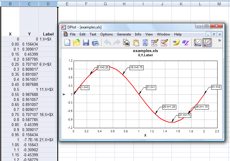
DPlot Windows software for Excel users to create presentation quality graphs

How to Add Data Labels in Excel - Excelchat | Excelchat After inserting a chart in Excel 2010 and earlier versions we need to do the followings to add data labels to the chart; Click inside the chart area to display the Chart Tools. Figure 2. Chart Tools. Click on Layout tab of the Chart Tools. In Labels group, click on Data Labels and select the position to add labels to the chart.

Working with Charts — XlsxWriter Documentation

Prevent Overlapping Data Labels in Excel Charts - Peltier Tech Data labels are terribly tedious to apply to slope charts, since these labels have to be positioned to the left of the first point and to the right of the last point of each series. This means the labels have to be tediously selected one by one, even to apply "standard" alignments.

How to create Custom Data Labels in Excel Charts • Efficiency 365

How to Place Labels Directly Through Your Line Graph in Microsoft Excel ... Right-click on top of one of those circular data points. You'll see a pop-up window. Click on Add Data Labels. Your unformatted labels will appear to the right of each data point: Click just once on any of those data labels. You'll see little squares around each data point. Then, right-click on any of those data labels. You'll see a pop-up menu.

How to Data Labels in a Bar Graph in Excel 2007 - YouTube

How to make a chart (graph) in Excel and save it as template 22.10.2015 · 3. Inset the chart in Excel worksheet. To add the graph on the current sheet, go to the Insert tab > Charts group, and click on a chart type you would like to create.. In Excel 2013 and Excel 2016, you can click the Recommended Charts button to view a gallery of pre-configured graphs that best match the selected data.. In this example, we are creating a 3-D …

How to Create a Bar Chart With Labels Above Bars in Excel

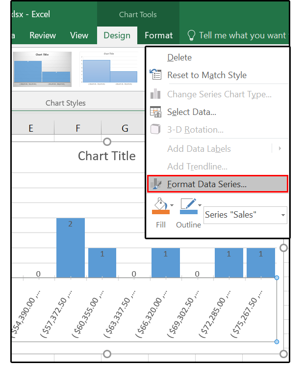
Excel Chart Data Labels - Microsoft Community Please verify that the range of data labels has been selected correctly. Right-click a data point on your chart, from the context menu choose Format Data Labels ..., choose Label Options > Label Contains Value from Cells > Select Range. In the Data Label Range dialog box, verify that the range includes all 26 cells.

Excel charts: add title, customize chart axis, legend and data labels

› Graph-Multiple-Lines-in-Excel3 Easy Ways to Graph Multiple Lines in Excel - wikiHow Nov 07, 2021 · Add your data into the column directly to the right of the last data column included in your graph. Be sure to title this column in row 1 so that it is labeled on the graph. You can create a new graph including this data by repeating the steps of highlighting a data set and inserting a line graph.

Data labels on Excel charts « projectwoman.com

Change the format of data labels in a chart To get there, after adding your data labels, select the data label to format, and then click Chart Elements > Data Labels > More Options. To go to the appropriate area, click one of the four icons ( Fill & Line, Effects, Size & Properties ( Layout & Properties in Outlook or Word), or Label Options) shown here.

How to create an Excel chart with no numerical labels? - Super User

How to create a chart with both percentage and value in Excel? After installing Kutools for Excel, please do as this:. 1.Click Kutools > Charts > Category Comparison > Stacked Chart with Percentage, see screenshot:. 2.In the Stacked column chart with percentage dialog box, specify the data range, axis labels and legend series from the original data range separately, see screenshot:. 3.Then click OK button, and a prompt message is popped out to remind you ...

34 Label Axis Excel Mac - Labels For Your Ideas

3 Axis Graph Excel Method: Add a Third Y-Axis - EngineerExcel Add Data Labels To a Multiple Y-Axis Excel Chart. Axis labels were created by right-clicking on the series and selecting “Add Data Labels”. By default, Excel adds the y-values of the data series. In this case, these were the scaled values, which wouldn’t have been accurate labels for the axis (they would have corresponded directly to the ...

Excel charts: add title, customize chart axis, legend and data labels

Add or remove data labels in a chart - support.microsoft.com Add data labels to a chart Click the data series or chart. To label one data point, after clicking the series, click that data point. In the upper right corner, next to the chart, click Add Chart Element > Data Labels. To change the location, click the arrow, and choose an option.

Science + Technology: Student Technology Usage Survey and Podcast

How to add or move data labels in Excel chart? - ExtendOffice In Excel 2013 or 2016. 1. Click the chart to show the Chart Elements button . 2. Then click the Chart Elements, and check Data Labels, then you can click the arrow to choose an option about the data labels in the sub menu. See screenshot: In Excel 2010 or 2007. 1. click on the chart to show the Layout tab in the Chart Tools group. See ...

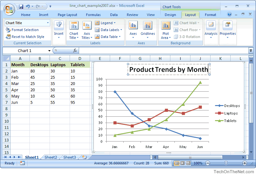
MS Excel 2007: How to Create a Line Chart

How To Use Dynamic Data Labels To Create Interactive Excel Charts To create a column chart with dynamic data labels, you need to follow these given steps. Select the data & Create a Combo Chart. Now select the column chart for revenue data and a line chart with marker for data labels Add Data Labels to the Line Chart With Marker. After then remove the Line Color and Marker Color.

Share :