41 excel chart add data labels
Add data labels and callouts to charts in Excel 365 - EasyTweaks.com Step #1: After generating the chart in Excel, right-click anywhere within the chart and select Add labels . Note that you can also select the very handy option of Adding data Callouts. How to create Custom Data Labels in Excel Charts - Efficiency 365 Create the chart as usual Add default data labels Click on each unwanted label (using slow double click) and delete it Select each item where you want the custom label one at a time Press F2 to move focus to the Formula editing box Type the equal to sign Now click on the cell which contains the appropriate label Press ENTER That's it.
Adding rich data labels to charts in Excel 2013 | Microsoft 365 Blog To add a data label in a shape, select the data point of interest, then right-click it to pull up the context menu. Click Add Data Label, then click Add Data Callout . The result is that your data label will appear in a graphical callout. In this case, the category Thr for the particular data label is automatically added to the callout too.

Excel chart add data labels
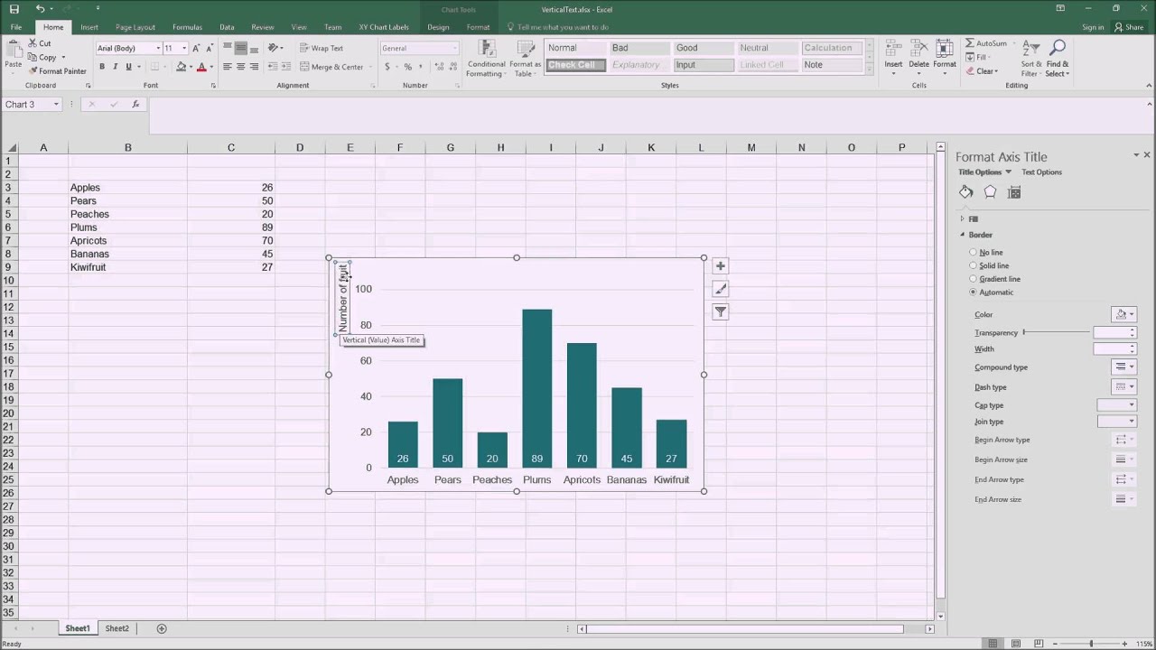
Add or remove data labels in a chart - support.microsoft.com Add data labels to a chart Click the data series or chart. To label one data point, after clicking the series, click that data point. In the upper right corner, next to the chart, click Add Chart Element > Data Labels. To change the location, click the arrow, and choose an option. › excel-chart-verticalExcel Chart Vertical Axis Text Labels • My Online Training Hub Apr 14, 2015 · To turn on the secondary vertical axis select the chart: Excel 2010: Chart Tools: Layout Tab > Axes > Secondary Vertical Axis > Show default axis. Excel 2013: Chart Tools: Design Tab > Add Chart Element > Axes > Secondary Vertical. Now your chart should look something like this with an axis on every side: How to Add Data Labels to an Excel 2010 Chart - dummies Select where you want the data label to be placed. Data labels added to a chart with a placement of Outside End. On the Chart Tools Layout tab, click Data Labels→More Data Label Options. The Format Data Labels dialog box appears.
Excel chart add data labels. How To Add Data Labels In Excel " .paymycheck The column chart will appear. For example, this is how we can add labels to one of the data series in our excel chart: Source: . Click the + symbol and add data labels by clicking it as shown below step 3: Click add chart element and select data labels, and then select a location for the data label option. Source: How to add or move data labels in Excel chart? - ExtendOffice To add or move data labels in a chart, you can do as below steps: In Excel 2013 or 2016. 1. Click the chart to show the Chart Elements button .. 2. Then click the Chart Elements, and check Data Labels, then you can click the arrow to choose an option about the data labels in the sub menu.See screenshot: support.microsoft.com › en-us › officeAdd a pie chart - support.microsoft.com To switch to one of these pie charts, click the chart, and then on the Chart Tools Design tab, click Change Chart Type. When the Change Chart Type gallery opens, pick the one you want. See Also. Select data for a chart in Excel. Create a chart in Excel. Add a chart to your document in Word. Add a chart to your PowerPoint presentation Edit titles or data labels in a chart - support.microsoft.com On a chart, click one time or two times on the data label that you want to link to a corresponding worksheet cell. The first click selects the data labels for the whole data series, and the second click selects the individual data label. Right-click the data label, and then click Format Data Label or Format Data Labels.
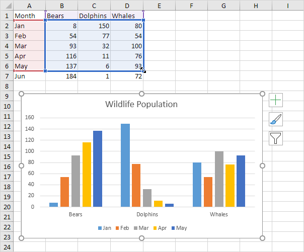
How to Use Cell Values for Excel Chart Labels - How-To Geek Select the chart, choose the "Chart Elements" option, click the "Data Labels" arrow, and then "More Options." Uncheck the "Value" box and check the "Value From Cells" box. Select cells C2:C6 to use for the data label range and then click the "OK" button. The values from these cells are now used for the chart data labels. Chart.ApplyDataLabels method (Excel) | Microsoft Docs ApplyDataLabels ( Type, LegendKey, AutoText, HasLeaderLines, ShowSeriesName, ShowCategoryName, ShowValue, ShowPercentage, ShowBubbleSize, Separator) expression A variable that represents a Chart object. Parameters Example This example applies category labels to series one on Chart1. VB Copy Charts ("Chart1").SeriesCollection (1). Add / Move Data Labels in Charts - Excel & Google Sheets Adding Data Labels Click on the graph Select + Sign in the top right of the graph Check Data Labels Change Position of Data Labels Click on the arrow next to Data Labels to change the position of where the labels are in relation to the bar chart Final Graph with Data Labels How To Create Labels In Excel - neighborsagainstmining.org Column names in your spreadsheet match the field names you want to insert in your labels. Right click the data series in the chart, and select add data labels > add data labels from the context menu to add data labels. In the mailings tab of word, select the finish & merge option and choose edit individual documents from the menu.
how to add data labels into Excel graphs - storytelling with data You can download the corresponding Excel file to follow along with these steps: Right-click on a point and choose Add Data Label. You can choose any point to add a label—I'm strategically choosing the endpoint because that's where a label would best align with my design. Excel defaults to labeling the numeric value, as shown below. How to add total labels to stacked column chart in Excel? - ExtendOffice 1. Create the stacked column chart. Select the source data, and click Insert > Insert Column or Bar Chart > Stacked Column. 2. Select the stacked column chart, and click Kutools > Charts > Chart Tools > Add Sum Labels to Chart. Then all total labels are added to every data point in the stacked column chart immediately. Custom Chart Data Labels In Excel With Formulas Follow the steps below to create the custom data labels. Select the chart label you want to change. In the formula-bar hit = (equals), select the cell reference containing your chart label's data. In this case, the first label is in cell E2. Finally, repeat for all your chart laebls. Add a DATA LABEL to ONE POINT on a chart in Excel Steps shown in the video above: Click on the chart line to add the data point to. All the data points will be highlighted. Click again on the single point that you want to add a data label to. Right-click and select ' Add data label ' This is the key step! Right-click again on the data point itself (not the label) and select ' Format data label '.
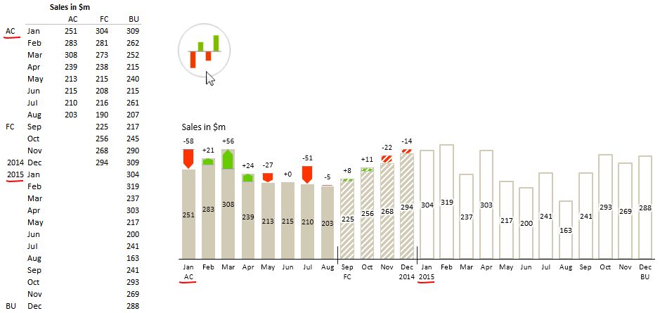
Variance analysis
Change the format of data labels in a chart To get there, after adding your data labels, select the data label to format, and then click Chart Elements > Data Labels > More Options. To go to the appropriate area, click one of the four icons ( Fill & Line, Effects, Size & Properties ( Layout & Properties in Outlook or Word), or Label Options) shown here.

How to create an Excel map chart
Adding Data Labels To An Excel Chart | MyExcelOnline In our example below, I add a Data Label to a column chart and then I format the data label using CTRL+1. I then select to custom format the numbers so it shows the values as thousands by adding a comma , after each zero and then showing the work k by adding "k". Example Custom Number Format: [$$-1004]#,##0 ,"k" ;- [$$-1004]#,##0 ,"k".

Excel Custom Chart Labels • My Online Training Hub
support.microsoft.com › en-us › topicPresent your data in a scatter chart or a line chart On the chart, click the legend, or add it from a list of chart elements (on the Design tab, click Add Chart Element > Legend, and then select a location for the legend). To plot one of the data series along a secondary vertical axis, click the data series, or select it from a list of chart elements (on the Format tab, in the Current Selection ...

How to Make Excel Charts More Intuitive by Adding Data Labels and Tables - Data Recovery Blog
How to add axis label to chart in Excel? - ExtendOffice Select the chart that you want to add axis label. 2. Navigate to Chart Tools Layout tab, and then click Axis Titles, see screenshot: 3.

How-to Use Data Labels from a Range in an Excel Chart - Excel Dashboard Templates
How to add data labels from different column in an Excel chart? Right click the data series in the chart, and select Add Data Labels > Add Data Labels from the context menu to add data labels. 2. Click any data label to select all data labels, and then click the specified data label to select it only in the chart. 3.
Creating a chart with dynamic labels - Microsoft Excel 2013
Add data labels to your Excel bubble charts | TechRepublic Right-click the data series and select Add Data Labels. Right-click one of the labels and select Format Data Labels. Select Y Value and Center. Move any labels that overlap. Select the data labels ...

Excel: How to make an Excel-lent bull's-eye chart
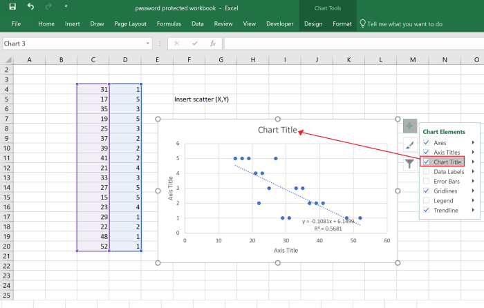
How To Add Data Labels In Excel " Gameps4 Then, click the insert tab along the top ribbon and click the insert scatter (x,y) option in the charts group. Click on the arrow next to data labels to change the position of where the labels are in relation to the bar chart. To format data labels in excel, choose the set of data labels to format. Source:
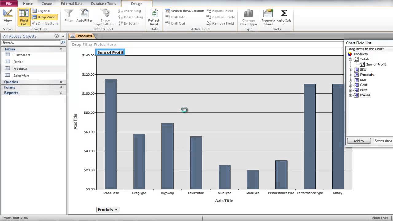
How to Create a Pivot Chart in Microsoft Access - YouTube
chandoo.org › wp › change-data-labels-in-chartsHow to Change Excel Chart Data Labels to Custom Values? May 05, 2010 · First add data labels to the chart (Layout Ribbon > Data Labels) Define the new data label values in a bunch of cells, like this: Now, click on any data label. This will select “all” data labels. Now click once again. At this point excel will select only one data label.

How to Add Data Labels in Excel - Excelchat | Excelchat
peltiertech.com › excel-column-Column Chart with Primary and Secondary Axes - Peltier Tech Oct 28, 2013 · The second chart shows the plotted data for the X axis (column B) and data for the the two secondary series (blank and secondary, in columns E & F). I’ve added data labels above the bars with the series names, so you can see where the zero-height Blank bars are. The blanks in the first chart align with the bars in the second, and vice versa.
Adding horizontally-aligned y-axis titles to charts in Excel 2016 - YouTube
How to Add Labels to Scatterplot Points in Excel - Statology Step 3: Add Labels to Points Next, click anywhere on the chart until a green plus (+) sign appears in the top right corner. Then click Data Labels, then click More Options… In the Format Data Labels window that appears on the right of the screen, uncheck the box next to Y Value and check the box next to Value From Cells.

Charting in Excel - Adding Data Labels - YouTube
How to Add Data Labels in Excel - Excelchat | Excelchat After inserting a chart in Excel 2010 and earlier versions we need to do the followings to add data labels to the chart; Click inside the chart area to display the Chart Tools. Figure 2. Chart Tools Click on Layout tab of the Chart Tools. In Labels group, click on Data Labels and select the position to add labels to the chart. Figure 3.

E-xcel Tuts: Add Data Labels to Excel Charts
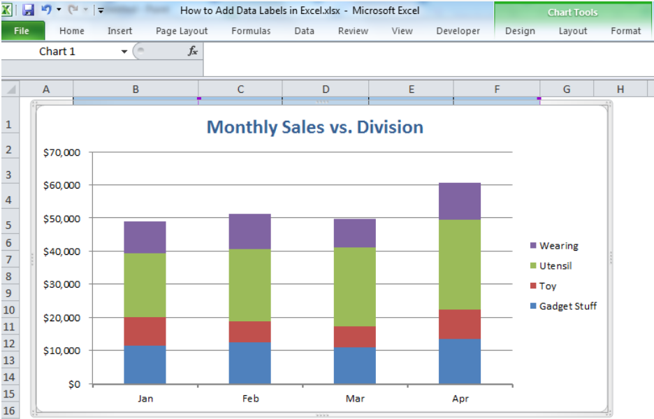
How to Add Total Data Labels to the Excel Stacked Bar Chart The basic chart function does not allow you to add a total data label that accounts for the sum of the individual components. Fortunately, creating these labels manually is a fairly simply process. Step 1: Create a sum of your stacked components and add it as an additional data series (this will distort your graph initially)

Adding Data Labels to Your Chart (Microsoft Excel)
How To Create Labels In Excel • winterhome The chart should look like this: The data labels for the two lines are not, technically, "data labels" at all. Source: db-excel.com. You will now finish the process and word will display the actual data for each label: How to add brackets to the existing code. Source: . Column names in your spreadsheet match the field names ...

Format Number Options for Chart Data Labels in PowerPoint 2011 for Mac
What Are Data Labels in Excel (Uses & Modifications) - ExcelDemy Follow the steps below to add data labels to an Excel chart. Steps: Please click on the data series or chart you wish to view. If you wish to label a single data point, click it again. Select Data Labels from the Add Chart Element menu (+) in the top right corner. By clicking the arrow, you can change the position.
How to Create a Scatter Plot in Excel - TurboFuture - Technology
How to Add Data Labels to an Excel 2010 Chart - dummies Select where you want the data label to be placed. Data labels added to a chart with a placement of Outside End. On the Chart Tools Layout tab, click Data Labels→More Data Label Options. The Format Data Labels dialog box appears.
Chart's Data Series in Excel - Easy Excel Tutorial
› excel-chart-verticalExcel Chart Vertical Axis Text Labels • My Online Training Hub Apr 14, 2015 · To turn on the secondary vertical axis select the chart: Excel 2010: Chart Tools: Layout Tab > Axes > Secondary Vertical Axis > Show default axis. Excel 2013: Chart Tools: Design Tab > Add Chart Element > Axes > Secondary Vertical. Now your chart should look something like this with an axis on every side:
How to Add Data Labels in Excel - Excelchat | Excelchat
Add or remove data labels in a chart - support.microsoft.com Add data labels to a chart Click the data series or chart. To label one data point, after clicking the series, click that data point. In the upper right corner, next to the chart, click Add Chart Element > Data Labels. To change the location, click the arrow, and choose an option.
Post a Comment for "41 excel chart add data labels"